

Time-series data arise in many fields including finance, signal processing, speech recognition and medicine. A standard approach to time-series problems usually requires manual engineering of features which can then be fed into a machine learning algorithm. Engineering of features generally requires some domain knowledge of the discipline where the data has originated from. For example, if one is dealing with signals (i.e. classification of EEG signals), then possible features would involve power spectra at various frequency bands, Hjorth parameters and several other specialized statistical properties.
A similar situation arises in image classification, where manually engineered features (obtained by applying a number of filters) could be used in classification algorithms. However, with the advent of deep learning, it has been shown that convolutional neural networks (CNN) can outperform this strategy. A CNN does not require any manual engineering of features. During training, the CNN learns lots of “filters” with increasing complexity as the layers get deeper, and uses them in a final classifier.
In this blog post, I will discuss the use of deep leaning methods to classify time-series data, without the need to manually engineer features. The example I will consider is the classic Human Activity Recognition (HAR) dataset from the UCI repository. The dataset contains the raw time-series data, as well as a pre-processed one with 561 engineered features. I will compare the performance of typical machine learning algorithms which use engineered features with two deep learning methods (convolutional and recurrent neural networks) and show that deep learning can approach the performance of the former.
I have used Tensorflow for the implementation and training of the models discussed in this post. In the discussion below, code snippets are provided to explain the implementation. For the complete code, please see my Github repository.
Convolutional Neural Networks (CNN)
The first step is to cast the data in a numpy array with shape (batch_size, seq_len, n_channels) where batch_size is the number of examples in a batch during training. seq_len is the length of the sequence in time-series (128 in our case) and n_channels is the number of channels where measurements are made. There are 9 channels in this case, which include 3 different acceleration measurements for each 3 coordinate axes. There are 6 classes of activities where each observation belong to: LAYING, STANDING, SITTING, WALKING_DOWNSTAIRS, WALKING_UPSTAIRS, WALKING.
First, we construct placeholders for the inputs to our computational graph:
graph = tf.Graph()

with graph.as_default():
    inputs_ = tf.placeholder(tf.float32, [None, seq_len, n_channels],
        name = 'inputs')
    labels_ = tf.placeholder(tf.float32, [None, n_classes], name = 'labels')
    keep_prob_ = tf.placeholder(tf.float32, name = 'keep')
    learning_rate_ = tf.placeholder(tf.float32, name = 'learning_rate')
where inputs_ are input tensors to be fed into the graph whose first dimension is kept at None to allow for variable batch sizes. labels_ are the one-hot encoded labels to be predicted, keep_prob_ is the keep probability used in dropout regularization to prevent overfitting, and learning_rate_ is the learning rate used in Adam optimizer.
The convolutional layers are constructed using one-dimensional kernels that move through the sequence (unlike images where 2d convolutions are used). These kernels act as filters which are being learned during training. As in many CNN architectures, the deeper the layers get, the higher the number of filters become. Each convolution is followed by pooling layers to reduce the sequence length. Below is a simple picture of a possible CNN architecture that can be used:
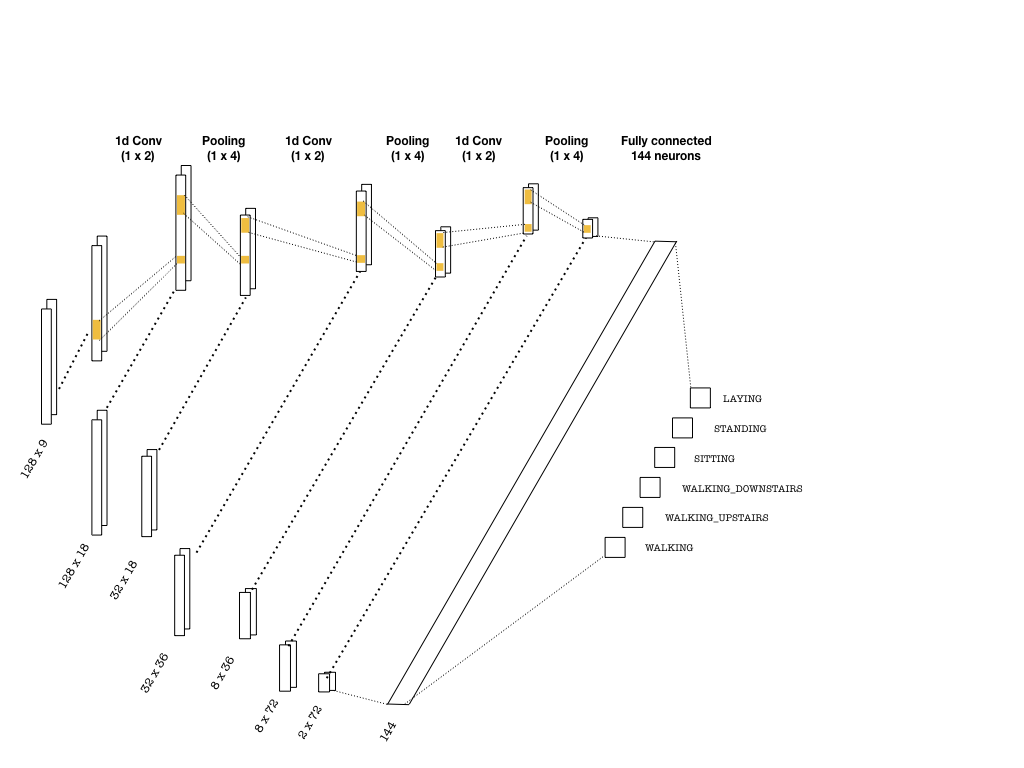
The convolutional layers that are slightly deeper than the ones depicted above are implemented as follows:
with graph.as_default():
    # (batch, 128, 9) -> (batch, 64, 18)
    conv1 = tf.layers.conv1d(inputs=inputs_, filters=18, kernel_size=2, strides=1,
        padding='same', activation = tf.nn.relu)
    max_pool_1 = tf.layers.max_pooling1d(inputs=conv1, pool_size=2, strides=2, padding='same')

    # (batch, 64, 18) -> (batch, 32, 36)
    conv2 = tf.layers.conv1d(inputs=max_pool_1, filters=36, kernel_size=2, strides=1,
    padding='same', activation = tf.nn.relu)
    max_pool_2 = tf.layers.max_pooling1d(inputs=conv2, pool_size=2, strides=2, padding='same')

    # (batch, 32, 36) -> (batch, 16, 72)
    conv3 = tf.layers.conv1d(inputs=max_pool_2, filters=72, kernel_size=2, strides=1,
    padding='same', activation = tf.nn.relu)
    max_pool_3 = tf.layers.max_pooling1d(inputs=conv3, pool_size=2, strides=2, padding='same')
# (batch, 16, 72) -> (batch, 8, 144)
    conv4 =tf.layers.conv1d(inputs=max_pool_3, filters=144, kernel_size=2, strides=1,
    padding='same', activation = tf.nn.relu)
    max_pool_4 = tf.layers.max_pooling1d(inputs=conv4, pool_size=2, strides=2, padding='same')
Once the last layer is reached, we need to flatten the tensor and feed it to a classifier with the right number of neurons (144 in the picture, 8×144 in the code snippet). Then, the classifier outputs logits, which are used in two instances:
- Computing the softmax cross entropy, which is a standard loss measure used in multi-class problems.
- Predicting class labels from the maximum probability as well as the accuracy.
These are implemented as follows:
with graph.as_default():
    # Flatten and add dropout
    flat = tf.reshape(max_pool_4, (-1, 8*144))
    flat = tf.nn.dropout(flat, keep_prob=keep_prob_)

    # Predictions
    logits = tf.layers.dense(flat, n_classes)

    # Cost function and optimizer
    cost = tf.reduce_mean(tf.nn.softmax_cross_entropy_with_logits(logits=logits,
        labels=labels_))
    optimizer = tf.train.AdamOptimizer(learning_rate_).minimize(cost)

    # Accuracy
    correct_pred = tf.equal(tf.argmax(logits, 1), tf.argmax(labels_, 1))
    accuracy = tf.reduce_mean(tf.cast(correct_pred, tf.float32), name='accuracy')
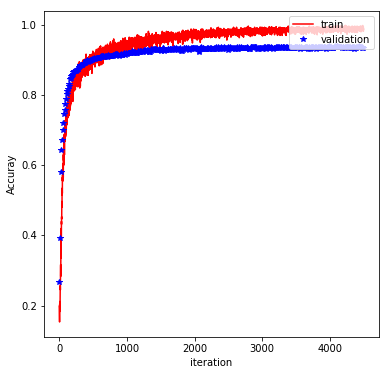
The rest of the implementation is pretty typical, and involve feeding the graph with batches of training data and evaluating the performance on a validation set. Finally, the trained model is evaluated on the test set. With the above architecture and a batch_size of 600, learning_rate of 0.0001, keep_prob of 0.5, and at 750 epochs, we obtain a test accuracy of 92%. The plot below shows how the training/validation accuracy evolves through the epochs:
Long-Short-Term Memory Networks (LSTM)
LSTMs are quite popular in dealing with text based data, and has been quite successful in sentiment analysis, language translation and text generation. Since this problem also involves a sequence of similar sorts, an LSTM is a great candidate to be tried.
Below is an example architecture which can be used in our problem:
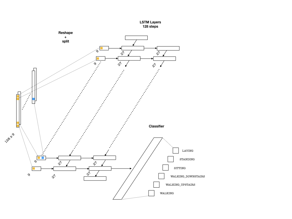
To feed the data into the network, we need to split our array into 128 pieces (one for each entry of the sequence that goes into an LSTM cell) each of shape (batch_size, n_channels). Then, a single layer of neurons will transform these inputs to be fed into the LSTM cells, each with the dimension lstm_size. This size parameter is chosen to be larger than the number of channels. This is in a way similar to embedding layers in text applications where words are embedded as vectors from a given vocabulary. Then, one needs to pick the number of LSTM layers (lstm_layers), which I have set to 2.
For the implementation, the placeholders are the same as above. The below code snippet implements the LSTM layers:
with graph.as_default():
    # Construct the LSTM inputs and LSTM cells
    lstm_in = tf.transpose(inputs_, [1,0,2]) # reshape into (seq_len, N, channels)
    lstm_in = tf.reshape(lstm_in, [-1, n_channels]) # Now (seq_len*N, n_channels)

    # To cells
    lstm_in = tf.layers.dense(lstm_in, lstm_size, activation=None)

    # Open up the tensor into a list of seq_len pieces
    lstm_in = tf.split(lstm_in, seq_len, 0)

    # Add LSTM layers
    lstm = tf.contrib.rnn.BasicLSTMCell(lstm_size)
    drop = tf.contrib.rnn.DropoutWrapper(lstm, output_keep_prob=keep_prob_)
    cell = tf.contrib.rnn.MultiRNNCell([drop] * lstm_layers)
    initial_state = cell.zero_state(batch_size, tf.float32)
There is an important technical detail in the above snippet. I reshaped the array from (batch_size, seq_len, n_channels) to (seq_len, batch_size, n_channels) first, so that tf.split would properly split the data (by the zeroth index) into a list of (batch_size, lstm_size) arrays at each step. The rest is pretty standard for LSTM implementations, involving construction of layers (including dropout for regularization) and then an initial state.
The next step is to implement the forward pass through the network and the cost function. One important technical aspect is that I included gradient clipping since it improves training by preventing exploding gradients during back propagation. Here is what the code looks like
with graph.as_default():
    outputs, final_state = tf.contrib.rnn.static_rnn(cell, lstm_in, dtype=tf.float32,
        initial_state = initial_state)

    # We only need the last output tensor to pass into a classifier
    logits = tf.layers.dense(outputs[-1], n_classes, name='logits')

    # Cost function and optimizer
    cost = tf.reduce_mean(tf.nn.softmax_cross_entropy_with_logits(logits=logits, labels=labels_))

    # Grad clipping
    train_op = tf.train.AdamOptimizer(learning_rate_)

    gradients = train_op.compute_gradients(cost)
    capped_gradients = [(tf.clip_by_value(grad, -1., 1.), var) for grad, var in gradients]
    optimizer = train_op.apply_gradients(capped_gradients)

    # Accuracy
    correct_pred = tf.equal(tf.argmax(logits, 1), tf.argmax(labels_, 1))
    accuracy = tf.reduce_mean(tf.cast(correct_pred, tf.float32), name='accuracy')
Notice that only the last last member of the sequence at the top of the LSTM outputs are used, since we are trying to predict one number per sequence (the class probability). The rest is similar to CNNs and we just need to feed the data into the graph to train. With lstm_size=27, lstm_layers=2, batch_size=600, learning_rate=0.0005, and keep_prob=0.5, I obtained around 85% accuracy on the test set. This is worse than the CNN result, but still quite good. It is possible that better choices of these hyperparameters would lead to improved results.
Comparison with engineered features
Previously, I have tested a few machine learning methods on this problem using the 561 pre-engineered features. One of the best performing models was a gradient booster (tree or linear), which results in an accuracy of %96 (you can read more about it from this notebook ).
Final Words
In this blog post, I have illustrated the use of CNNs and LSTMs for time-series classification and shown that a deep architecture can approach the performance of a model trained on pre-engineered features. Deep learning models “engineer” their own features during training. This is highly desirable, since one does not need to have domain expertise from where the data has originated from, to be able to train an accurate model. With more data, and further hyperparameter tuning, it is possible that deep learning methods can surpass the models trained on pre-engineered features.
The sequence we used in this post was fairly small (128 steps). One may wonder what would happen if the number of steps were much larger and worry about the trainability of these architectures I discussed. One possible architecture would involve a combination of LSTM and CNN, which could work better for larger sequences (i.e. > 1000, which is problematic for LSTMs). In this case, several convolutions with pooling can effectively reduce the number of steps in the first few layers and the resulting shorter sequences can be fed into LSTM layers. An example of such an architecture has recently been used in atrial fibrillation detection from mobile device recordings.
Note: In the previous version of this post, the reported test accuracies were higher. This was due to a bug in the code during reading the train/test sets.
Links
- Also see G. Chevalier’s repo and A. Saeed’s blog where I got lots of inspiration.
- Repository containing LSTM and CNN codes
- Repository containing several models trained on 561 manually generated features (in R)
- A notebook on the analysis of the data and predictions with gradient boosters (in R).

Hello,
I just wanted to thank you for your efforts in preparing this blog post. I have searched on and on, and as of yet, your post contains the clearest explanation of the internal manipulations taking place in learning LSTM networks.
Thank you!
LikeLiked by 1 person
Thanks! I am glad you enjoyed the post.
LikeLike
In your complete code,when train the network, how the function get_batches(x_tr,y_tra,batch_size) from and work here? hope your reply!
LikeLike
That function builds batches from the given data. We do not feed the whole training set into the network, instead we feed it piece by piece which is what this function does.
LikeLike
Thank you very much for this post. But, I got this error: ModuleNotFoundError: No module named ‘utils.utilities’. can you tell me how to fix this
LikeLike
Thanks! This error says that the folder utils is not in your working directory. Make sure it is there and the problem will disappear. That folder contains the file ‘utilities.py’ which is needed.
LikeLike
Hi, how do you draw these neat figure for networks?
THanks
LikeLike
I used keynote in Mac, it is similar to powerpoint.
LikeLike
Would this scenario make sense to use Conv1d?
Suppose I want to do time series classifiaction with tf/keras and use conv1d, where my original data has shape 500 samples, by 12 features. In my case, I have 500 separate time series observations each with 12 time points. In my case the 12 is months of the year. I have 500 observation of 12 months so my data has shape 500×12.
How would I do this with Conv1D? In my case I don’t have any “channels” like your example so would a 1D conv still make sense?
LikeLike
If so How to use it? Similar as above? any modifications need to be made?
LikeLike
The data size seems to be too small (only 500 instances) to use a convolutional network. I would recommend using a much simpler model (maybe some linear model) which will be more useful.
If you had many more samples, you can try to use a convolutional network, with only one channel initially. In the layers, you will end up with filters that will map this 1 channel into multiple ones and could potentially learn the patterns in the time series.
LikeLike
OK in my case suppose I have 10000K such samples in my Case now I have 100K by 12K input matrix.
Suppose my first layer is a Conv1D with 10 filters and kernel size of 4 and stride 1. Is my expected output shape supposed to be
100K by 9 by 10channels?
LikeLike
The expected output shape depends on the way the convolutional layer is chosen. If you choose “same” as padding, then the convolutional layer will map a shape (batch_size, 9, 1) –> (batch_size, 9, 10). Here batch_size is the number of data instances you use for each step of the training of the network (<= 100k). If you use "valid" padding, I believe it depends on the implementation, but you will end up with either (batch_size,3,10) or (batch_size,2,10). My recommendation would be to use "same" padding and then use maxpool layers to reduce the size further.
LikeLike
Please see my comment below. Critical to my problem. Thank you
LikeLike
Hi,
A quick question: why is the test accuracy almost 5% lower than the validation accuracy? Is that acceptable? Given the data is of the same nature, shouldnt we expect very simialr accuracy?
LikeLike
I meant the CNN case …
LikeLike
Test accuracies are usually lower than validation, since the validation set is used to find the hyperparameters. When a new set of observations (test set) are supplied, the model does slightly worse. Having said that, I did not spend too much time tuning the hyperparameters (like the size and number of layers). If one carefully tunes them, the difference between validation and test error will likely reduce.
LikeLike
I agree that if we were setting hyper parameters then test accuracy would have been lower. But here we don’t. Validation set doesn’t influence the computations as it just sits there and we only use it to track the accuracy. I feel that here the test set is provided by uci and probably has a different nature in terms of measurement noise etc. I did a simple test in which I split the provided training data to test as validation sets and then the outcome accuracy becomes similar.
LikeLike
Correction: split the provided training data to test *and validation
LikeLike
The notebook in the post shows training only with one set of hyperparameters. However, to find that set, I tried a bunch of them manually (size and number of hidden layers, learning rate, number of epochs etc.) and then picked a set that gave the best validation accuracy. So, I used the validation set to pick them. I believe that with a better choice of hyperparameters (maybe simply by reducing the number of epochs) the test and validation accuracy will become closer.
LikeLike
You say that you tried bunch of them manually. Isn’t it possible to tune those parameters using scikti learn (or caret for R) or even Tensorflow or Keras?
LikeLike
I think it should be possible to use gridcv in scikit-learn or caret in R to try a bunch of hyperparameters and find the best subset by cross validation. I am not sure whether wrappers for tensorflow or keras models are currently available for that purpose. However, in training deep neural networks, one generally relies on manual selection of hyperparameters, since the training itself takes a long time. Given that there are many hyperparameters to tune, an exhaustive search (like in caret of scikit-learn) would be very time consuming. Usually, one can follow how the training goes and stop if necessary and re-tune the parameters to start over. After some experimentation, such a procedure generally works well.
LikeLike
OK Thanks. One more thing specific about what I have in mind to do. My dataset is basically 6 channels, or to be more precise, 6 different measurement types at different locations where at each location the length of the records can be different to the others. So I have concatanted them all and hence I will end up with 6 channels of very long records (could be 10000 or much more samples). What is your advice to use/modify the CNN code you have provided?
LikeLike
I am not sure I understand the problem correctly, but I will try to reply as best as I can. If the sequence length is too large, than you may need to choose a very small batch size to fit the arrays in the memory. This may cause problems and you may not even train the network properly. One option would be to divide the sequence into blocks and treat each block as a separate data instance. I have done something similar in this link: https://github.com/bhimmetoglu/datasciencecom-mhealth/blob/master/post.md
Hope this helps
LikeLike
Hi Burak,
Thanks for your post. It was extremely helpful.
Sorry if this is a duplicate question, but I have been trying to save the trained model to disk, and noticed that you already do it. However, when trying to read it back from the files, using
with tf.Session(graph=graph) as sess:
# Restore
saver.restore(sess, tf.train.latest_checkpoint(‘checkpoints-cnn’))
I get “No variables to save”, when trying to create the saver object. Could you point me in the right direction?
Thanks!
LikeLike
Hi falza,
Before restoring the graph, you should train and save it. If you have already done that, there may be a small bug in your code. There is an entry in stackoverflow about this, maybe that would help:
https://stackoverflow.com/questions/36281129/no-variable-to-save-error-in-tensorflow
LikeLike
Hi,
when running the HAR-LSTM notebook example, I get the following error message:
—————————————————————————
ValueError Traceback (most recent call last)
in ()
24
25 loss, _ , state, acc = sess.run([cost, optimizer, final_state, accuracy],
—> 26 feed_dict = feed)
27 train_acc.append(acc)
28 train_loss.append(loss)
~/anaconda3/envs/machine/lib/python3.6/site-packages/tensorflow/python/client/session.py in run(self, fetches, feed_dict, options, run_metadata)
893 try:
894 result = self._run(None, fetches, feed_dict, options_ptr,
–> 895 run_metadata_ptr)
896 if run_metadata:
897 proto_data = tf_session.TF_GetBuffer(run_metadata_ptr)
~/anaconda3/envs/machine/lib/python3.6/site-packages/tensorflow/python/client/session.py in _run(self, handle, fetches, feed_dict, options, run_metadata)
1063 feed_handles = {}
1064 if feed_dict:
-> 1065 feed_dict = nest.flatten_dict_items(feed_dict)
1066 for feed, feed_val in feed_dict.items():
1067 for subfeed, subfeed_val in _feed_fn(feed, feed_val):
~/anaconda3/envs/machine/lib/python3.6/site-packages/tensorflow/python/util/nest.py in flatten_dict_items(dictionary)
249 raise ValueError(
250 “Could not flatten dictionary: key %s is not unique.”
–> 251 % (new_i))
252 flat_dictionary[new_i] = new_v
253 return flat_dictionary
ValueError: Could not flatten dictionary: key Tensor(“MultiRNNCellZeroState/DropoutWrapperZeroState/LSTMCellZeroState/zeros:0”, shape=(600, 27), dtype=float32) is not unique.
Can you help me with that?
Best regards
Alex
LikeLike
Could you let me know the version of tensorflow you are using?
LikeLike
Thanks for your answer. I am using version 1.5, maybe it is because of the recent changes?
Best regards and thanks again for the article
Alex
LikeLike
Possibly. I used version 1.0. I will give a look
LikeLike
Thanks for sharing nice work… I would like to use tensor flow for classification of time series of satellite image… I want to know how to use 2d convolutions as u have mentioned in you post… Kindly guide me…
LikeLike
2d image classification is a more well-known application for convolutional nets. For satellite data, you can give a look at kernels at some Kaggle competitions. For example:
https://www.kaggle.com/c/dstl-satellite-imagery-feature-detection
https://www.kaggle.com/rhammell/ships-in-satellite-imagery
LikeLike
Hi,
Thanks for writing this article – very interesting. I have a question about the data standardization that you have done before feeding to the NN. It looks like from the code that you are computing the average and standard deviation over the zeroth index of the array which corresponds to the index of the training examples. Does this mean that the data are being scaled by different amounts for different time steps?
Intuitively, I thought that it would make more sense to scale all of the data for the 128 time steps for a given training example by the same amount, and thus not change their relative values.
Thanks for your time,
LikeLike
Yes, I compute the average across samples, so that I normalize variation between them. to [-1,1]. You can definitely try to normalize the signal across the time axis. I haven’t tried that but, it is worth looking at.
LikeLike
Hi there,
First of all, thanks and congrats for the post.
I would love to know, if you have time, which would be the proper way to improve the data feeding by substitute the feed_dic with queues. (Similar to https://github.com/tensorflow/models/blob/master/tutorials/image/cifar10/cifar10.py)
Being the data composed from different files, which would be the proper way to do it? Would there be a penalization using data from several files to compose the data feed to a single branch data block?
Again, thanks and regards
LikeLike
Hi, sorry for the late reply. I am not really sure what the answer would be. I always use feed_dicts, since they have worked for me. If I understand your question correctly, you are trying to load the data from disk into the batch, instead of pulling it from memory. Then, there will be the i/o overhead of reading from file, which will slow down training. Is that what you are asking?
LikeLike
Hi!
According to TF’s recommendations, it is preferred to use Datasets and queues feeding the data, as they employ multiple threads to efficiently feed the data pipeline. Therefore a thread handles the IO and the data flows smoothly. An example can be seen at https://github.com/tensorflow/models/blob/master/tutorials/image/cifar10/cifar10.py
I also usually use feed_dic, but thinking about the problem, I doubt how to implement this data queue when several files need to be read at the same time (each with one channel info).
I managed to implement a first approach but it behaved poorly, being the performance really bad. So just wondering how would you adapt https://github.com/healthDataScience/deep-learning-HAR/blob/master/utils/utilities.py.
Regards
LikeLike
Not really sure. I haven’t thought about this before so I don’t have a good answer
LikeLike
Really appreciate such an awesome work. One question after reading your code. In utils python file you have a function called standarize that normalize train and test datasets, I saw you use their own means and standard deviations to normalize both sets.
But I have been taught that when normalizing train and test dataset, test must be normalized with train mean and sd.
What is the reason of doing it that way?
Thanks in advance.
LikeLike
Hi Oscar,
I’am glad the post was useful.
You are right, the normalization should be performed the way you describe. This is a bug in the code (among others related the compatibility with latest tensorflow) will be fixed when I have time.
Thanks for reporting,
Burak
LikeLike
Amazing work, thank you for writing this article !!! I just wanted to ask you about the following line:
lstm_in = tf.layers.dense(lstm_in, lstm_size, activation=None)
Why do we need to use a single layer neurons to transform inputs to be fed into the LSTM cells? You mentioned that this is similar to embedding layers in text applications, but in text application we apply embedding layer to represent each word with a bunch of numbers (corresponding to those words), and here you already dealing with time series which are numbers. Can you please explain ?
LikeLike
Hi Amir,
Thanks for your comment, I am glad the post was useful.
This step allows you the “feature extraction” feature of the LSTM. From 9 channels, we pass to a 27 dimensional representation at each time-step by this layer. This allows more complex structures/features to be learned from the 9 measurements. You can experiment with the dimension of this layer (27) to see how the results will change.
This is a bit different from language applications where the dimensionality of vocabulary is much larger than 9. So the embedding step has a different meaning (it reduces the dimensionality of word vectors). However, the idea is kind of analogous.
LikeLike
Thank you for a prompt answer. Yeah I understood it, in addition to reshaping the final output of the CNN to be compatible with the number of LSTM units you also try to keep the information about the time dependencies and let the model to learn which one of the channels is more important at each time instance ,aka feature extraction. Very clever!!!!
LikeLike
Merhaba Burak,
Thanks for your great post! Do you have any other example with “multi-time series with a multi-class problem? I would try to see how to plugin features into to the multi-series in a model (features providing the correlation with 3-4 series)
Regards
LikeLike
Merhaba Murat,
Glad you found the post useful. The following link contains an analysis for a similar dataset:
https://github.com/bhimmetoglu/datasciencecom-mhealth
The difference in this one is that the time series is much longer, and the strategy is to break it apart into pieces.
I would also recommend datasets from physionet.org, where you can find lots of interesting medical time series data (ECG, EKG etc.)
Hope this helps
LikeLike
Hi Burak,
Thanks for your awesome post. In G. Chevalier’s repo, weights and biases defined as below.
Why don’t you use weights and biases ?
# Graph weights
weights = {
‘hidden’: tf.Variable(tf.random_normal([n_input, n_hidden])), # Hidden layer weights
‘out’: tf.Variable(tf.random_normal([n_hidden, n_classes], mean=1.0))
}
biases = {
‘hidden’: tf.Variable(tf.random_normal([n_hidden])),
‘out’: tf.Variable(tf.random_normal([n_classes]))
}
LikeLike
Hi Aslihan,
I’m glad the post was useful.
I use the tf.layers.dense module, which initializes weights and biases automatically (https://www.tensorflow.org/api_docs/python/tf/layers/dense). So, I believe the implementation should be equivalent.
Hope this helps,
Burak
LikeLike
Hi Burak,
Thank you for your answer. I’m confused about initial state. When I initialize state with using,
initial_state = cell.zero_state(batch_size, tf.float32), I can’t predict with a single sample (batchsize=1). It gives error that the size of the batch I use for prediction does not match the training batch size. When I close initial state, I can predict with batchsize=1.
G. Chevalier doesn’t initialize state. He just use state_is_tuple=True.
lstm_cell = tf.contrib.rnn.BasicLSTMCell(n_hidden, forget_bias=1.0, state_is_tuple=True)
I also looked Aymeric Damien’s examples (https://github.com/aymericdamien/TensorFlow-Examples/blob/master/examples/3_NeuralNetworks/recurrent_network.py) and he doesn’t initialize states. Should I initialize states with cell.zero_state or does lstm do it automatically in itself ? I’m really confused about this problem.
LikeLike
Hi Aslihan,
Not sure why you get an error with batchsize=1. Maybe there is a mismatch in the shape of the tensor when passed to zero_state.
Having said that, the LSTM part of my implementation was using an older version of tensorflow. When I tried to run the same code in the latest tensorflow a while back, I got some other errors. I will look into it in more detail when I get the time to do it. Maybe it is related to this issue (don’t remember the details now).
Maybe just remove the zero state for the moment, since you really don’t need it (that term is a bias, and if you don’t specify it, the weights will be initialized with zeros).
LikeLike
Is there a way to plot time series for each human activity they belong?
LikeLike
Yes, it should be possible. Just take a subset of the data which belongs to a given activity. Then, you can plot them.
LikeLike
I’m really newbie to Python and Tensorflow library. Can you help me with some examples or some guide with which I could practice? Thank you
LikeLike
Hi Liugi,
There are a lot of great online resources to learn Python and Tensorflow. I would recommend datacamp and coursera as a start. If you have specific questions about this post, I would be happy to answer them.
LikeLike